Current-induced zero-field domain wall depinning in cylindrical nanowires

Magnetic states

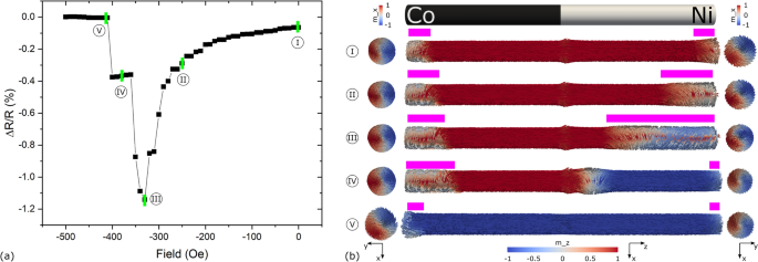
The presence of a DW or a non-axial magnetic configuration along the NW was measured using the anisotropic magnetoresistance (AMR) effect. The AMR depends on the direction of the measurement current with respect to the one of the magnetization¹³. Therefore, simplifying, it gives an overall measure of the portion of the NW’s magnetization M that is not parallel to the direction of the applied measurement current I_m. At ± 3 kOe (and remanence due to high shape anisotropy), most of the NW’s magnetization is in the same direction as the measurement current, i.e., along the NW’s long axis, resulting in saturated high resistance states, such as states I and V in Fig. 1. This figure shows a simulated AMR curve of a Co/Ni NW starting from remanence (state I) and increasing the field towards the negative direction until the NW’s magnetization is reversed (state V). Side views consisting on cross sections and sparse glyph representations of the selected magnetization states I to V in Fig. 1a are shown in Fig. 1b with the Co on the left and Ni on the right. Starting at remanence (state I), as the field increases, magnetization vortices appear at the ends of the NW, driving magnetization away from the axial direction and resulting in lower resistance states, as is shown in states II and III in Fig. 1 with a qualitative measure of the vortices indicated with pink bars above the NW side views in Fig. 1b.

These vortices minimize the magnetostatic energy. As the external applied field increases, the vortices grow larger in Ni, since its saturation magnetization, exchange energy and magneto crystalline anisotropy are at least one order of magnitude less than the ones of Co, i.e., it is a “softer” magnetic material. Notice also that this happens regardless of both having the same shape anisotropy (same geometry). When the vortices reach a critical “size” at a certain field, as shown in state III of Fig. 1, a DW nucleates and propagates from the right (Ni) end and is pinned at some point within the Ni segment close to the interface¹⁴, increasing the axial component of the magnetization as indicated by state IV (a detailed view of the DW can be found in supporting Fig. S1). Finally, when the field is further increased, the DW de-pins and propagates to the opposite (Co) end, leaving most of the magnetization in the axial direction again, as indicated by state V in Fig. 1. Note that NWs with vortices at their ends and pinned DWs within their length have a lower resistance, compared to uniformly-magnetized NWs, as they contain magnetization textures out of axis.

For the experimental study, the system had to first be brought to state IV of Fig. 1. This was achieved by saturating the magnetization by applying + 3 kOe, decreasing the field, inverting it and increasing it only until the first resistance jump was reached. Once in this state, the magnetic field was ramped down to zero, where two scenarios could occur: either the magnetization reversed to state I, i.e., the DW “returned” to where it was nucleated from, or the DW remained pinned in state IV of Fig. 1 at zero field. After returning the field to zero from state IV, a way to test for the outcome of these scenarios was to ramp the field up again in the negative direction. If the magnetization returned to state I, two resistance jumps would be observed in the AMR curve: one related to the transition from state III to state IV and one related to the transition from state IV to state V. On the other hand, if the DW remained pinned, i.e., state IV was conserved at zero field, once the field ramps up again, only the resistance jump related to the transition from state IV to V would be observed. As will be seen from all measurements in the following sections and in supporting Figs. S3, S4, after being pinned (state IV), the DW never returned to state III after reducing the field to zero, i.e., only one resistance jump was always observed when ramping the field up again. In addition to this, if the DW remained pinned at zero field and a current pulse was used to induce its de-pinning, i.e., take the magnetization to state V, no resistance jump would be observed once the field was ramped up again.

Nanowire composition

The nanowire composition was first investigated using energy-dispersive X-ray (EDX) spectroscopy within a scanning electron microscope (SEM), while they were inside the membrane to examine their total length and the lengths of the segments. These spectra were then compared to the lengths of the released, contacted NWs to infer their segments length. Figure 2 shows the SEM images of the contacted (a) Ni/Co/Ni and (b) Co/Ni NWs (top), as well as their respective EDX spectra (bottom).Measuring the portions at the positions where the Co and Ni spectra cross, we found the lengths of the segments of Ni/Co/Ni as [3.37/7.31/3.64] µm (Fig. 2a) and of Co/Ni as [13.96/11.71] µm (Fig. 2b). The average diameters were found to be 188 nm and 148 nm for the three- and two-segmented NWs in Fig. 2a,b, respectively. These values were used to calculate the current densities applied both for the continuous AMR measurements and pulse amplitudes.

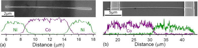
Scanning electron microscope image (top) and composition spectra (bottom) of (a) Ni/Co/Ni and (b) Co/Ni nanowires.

Three-segmented nanowire

Current pulses at zero field were first tested in the Ni/Co/Ni NW, shown in Fig. 2a, where previous experiments showed that, compared to two-segmented NWs, state IV persisted for higher negative fields before switching to state V as the field was ramped up (the “plateau” was wider)¹⁵. Furthermore, the pinning event (state IV) was more evident in the resistance value (discernible from states III and V) of the AMR curve compared to two-segmented NWs. The normalized AMR values from such NW, with its long axis parallel to the applied field, and in a range relevant to the pinning/de-pinning events is shown in Fig. 3 (solid line). This curve starts from a saturated magnetization state in the “right” direction (+ 3 kOe, not shown) and proceeds to a saturated state in the “left” direction (− 3 kOe, not shown), as indicated by the arrow at the bottom (for a full curve, see Supplementary Fig. S2).

Using the method described before, the NW was brought to a magnetic state in which a DW was pinned, as seen in Fig. 3a, red open squares (equivalent to state IV in Fig. 1). After this, the field was reduced to 0 ± 5 Oe (open blue triangles in Fig. 3a) where current pulses of different magnitudes were applied before ramping the field up again to find out about the resulting magnetization state. The outcome of two representative pulses is displayed in Fig. 3b: after a current pulse of 9.21 × 10¹¹ A/m² and 10 ns width was applied (solid red squares), one resistance jump was observed during the field ramp up, meaning that the applied pulse did not induce the de-pinning of the DW. On the other hand, after a current pulse of 1.38 × 10¹² A/m² and 20 ns width was used, neither of the resistance jumps were observed, meaning the magnetization assumed a state equivalent to state V in Fig. 1, i.e., the current pulse induced the de-pinning of the DW, reversing the magnetization.

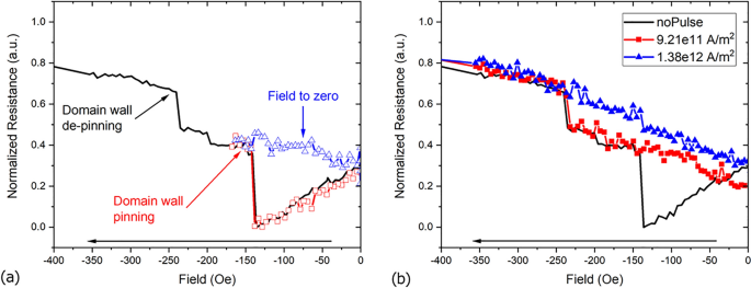
(a) Anisotropic magneto-resistance measurement of Ni/Co/Ni cylindrical nanowire with a pinned domain wall and the subsequent reduction of the external field to zero, after which nanosecond square current pulses were applied. (b) Magnetoresistance profile after two different current pulses were applied at zero field: 9.21 × 10¹¹ A/m², 10 ns width (red squares), the de-pinning resistance jump indicates the domain wall was not de-pinned; 1.38 × 10¹² A/m², 20 ns (blue triangles) results in the de-pinning of the DW as the depinning resistance jump is not observed.

One way to quantify the effect of the current pulses is to plot the gradient of the AMR curves in Fig. 3b against the applied field and identify the peaks at the fields at which the resistance jumps occurred, as shown in Fig. 4. From Fig. 4, when no pulse was applied, two peaks at approx. − 140 and − 240 Oe are displayed, corresponding to the resistance jumps of the black solid line in Fig. 3b. When the current pulse did not induce the de-pinning of the DW (solid red squares in Fig. 4), only the peak around − 240 Oe can be observed, corresponding to the de-pinning resistance jump in Fig. 3a. On the other hand, when the current pulse induced the de-pinning of the DW (solid blue triangles in Fig. 4), no distinct peak can be seen over the noise. For this three-segment NW, all measurements can be found in the Supplementary Fig. S3.

In the three-segmented NW presented, it is possible for two DWs to be pinned near the two Ni/Co interfaces at the same time although, realistically, due to imperfections such as different geometries at the NW ends¹⁶, one DW would nucleate. This makes it difficult to track which segments are being switched, i.e., which DW is moving and in which direction as both may be moving and collapsing into each other at the same time when the de-pinning jump is observed. This difficulty in tracking the DW gets more complex as the number of segments increases because the AMR value of multiple-pinned DWs does not vary greatly, when only one DW de-pins¹⁵.

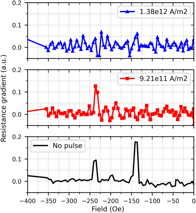
Numerical gradients of the resistances obtained from the curves in Fig. 3b.

Two-segmented nanowire

In order to track a single DW, the described method was applied to the two-segmented Co/Ni NW, shown in Fig. 2b, where only one DW can be pinned, and whose magnetization states correspond to the ones presented in Fig. 1. The experiment was setup in a way that for a “Positive” current pulse, electrons flowed from left to right (from Co to Ni) while for a “Negative” current pulse, electrons flowed from right to left (from Ni to Co). Figure 5 shows the observed fields at which a peak appeared in the gradient of the AMR curves, after current pulses of 1 × 10¹² A/m² with different pulse widths and polarities were applied. The appearance of the peaks means the current pulses did not induce the de-pinning of the DW (all measurements can be found in the Supplementary Fig. S4). As seen in Fig. 5 (and Supplementary Fig. S4) for pulses of 22 ns and longer, domain wall de-pinning was observed for positive but not for negative current pulses, i.e., the de-pinning event was dependent on the direction of the applied current pulse and only happened when electrons flowed from Ni to Co.

In addition to this, Fig. 5 also shows that the de-pinning field value differs by around 40 Oe for some measurements (from around − 215 to − 260 Oe). This difference was also found in measurements performed without applying current pulses in two and three-segmented NWs and can be found in the Supplementary Fig. S5a,b for two and three-segmented NWs, respectively.

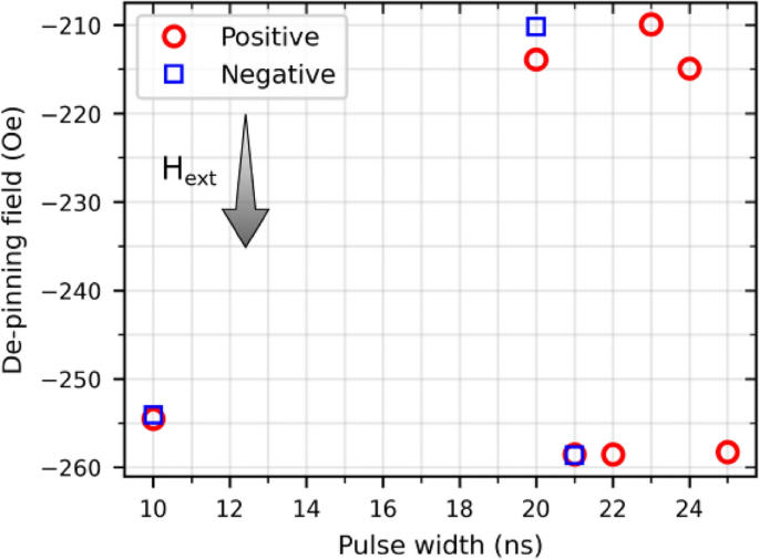
De-pinning field observed after applying pulses of 1 × 10¹² A/m² and different pulse widths and polarities. For pulse widths longer than 22 ns, negative pulses induce the de-pinning of the DW and no de-pinning field is observed.

Current-induced heating

In addition to the current pulses, as the NW was constantly under an applied measurement current of 2 × 10⁸ A/m², to measure the AMR, heating was expected to emerge to some extent. For every measurement in which a pulse was applied, a measurement without a pulse was first conducted in order to check for any changes in the DW pinning field and as an additional reset of the NW (saturating to + 3 kOe in every measurement was considered as a reset). AMR measurements took 30 min each, when no pulse was applied and 39 min when pulses were applied (additional time was needed to return the field to zero and ramp it back up again after the pulse was applied). Overall, the two-segmented Co/Ni NW was under constant applied current for a total of 20.7 h.

The last day of measurements is summarized in Fig. S6, where the minimum resistance, extracted from all reported AMR curves, is shown. It is seen that each subsequent measurement increases the minimum resistance and that the system does not completely cool down in the time needed to input new parameters for the next experiment (some seconds to minutes). The reset to minimum resistance only happened when the system was allowed to cool down overnight.