Sample structure and magnetic properties
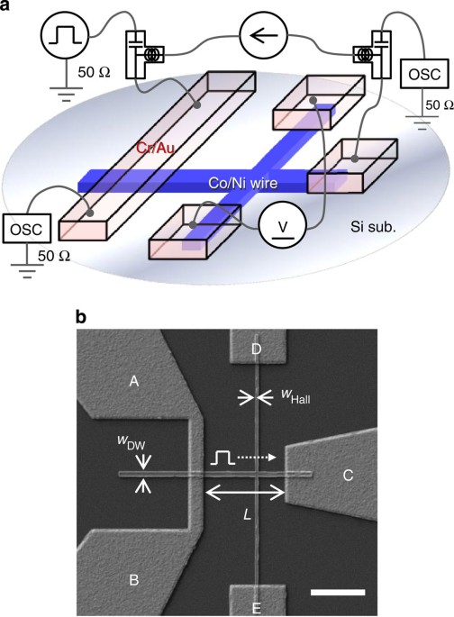
For DW stabilization experiments, multiple perpendicularly magnetized Co/Ni layers are used18 was used deposited on Si substrate. This is a promising material for application to DW motion devices due to it having several advantages in terms of stable operation and retention properties21,22,23due to its nature that the DW can be driven by an adiabatic STT22. By measuring the overall film magnetization curves along both the in-plane and out-of-plane directions, the saturation magnetization was obtained MQthe vertical anisotropy constant and the forced field were obtained to be 0.96 T, 6.1 × 10⁵JM-3and 16.5 metric tons, respectively, which are consistent with the values reported in previous works21,22,23,24. The deposited film was patterned into a cross-shaped nanowire with a width of 160 nm, to which four Cr/Au electrodes (A–B, C, D, and E) were attached (Figure 1). The direction of magnetization around the Hall junction of the nanowires was detected by measuring the Hall resistance through the exceptional Hall effect. To prepare the DW in the nanowire, after the magnetization was saturated with a large out-of-plane magnetic field, a current pulse was applied to the Cr/Au electrode (A to B) under an out-of-plane auxiliary field. HAwhere the current pulse generates a local Oersted field, which forms a reflection field. All measurements were performed at room temperature. (See Figure 1a For experimental setup and methods to obtain detailed information about sample preparation and measurement.)
(A) Schematic diagram of the structure of the device with the measuring circuit used to measure DW determination. (for) Top view of a manufactured device taken with a scanning electron microscope. Scale bar is 2 µm. DW motion area display, ThDeutsche WelleThat of the hall probe, Thhallthe length between the interconnection A – B and pole C, towere designed to be 160 nm, 80 nm, and 3 µm, respectively.
Figure 2a,b Show resistance versus out-of-plane magnetic field (R–H) Curves for nanowires without and with DW, respectively. The insets show the corresponding magnetization configurations. Major R–H Curve in Figure 2a It shows a square hysteresis, indicating a smooth vertical axis for the current Co/Ni wire. The coercive field, which corresponds to the core field of magnetic fields, is about 350 mT. Figure 2b Displays 10 independent R–H Curves measured after DW preparation. the R–H The curves obtained with no HA (labeled I) shows sudden jumps in a sweeping field of about +20 and +35 mT. The former and latter fields correspond to the DW propagation field in the straight region and the transgression field in the right direction at the Hall junction, respectively18. On the basis of this result, HA +27 mT was used to initialize the DW to the left of the Hall junction, prior to all currently induced DW removal measurements shown below. The negative field scan starting in this initial state (labeled II) shows a drop in resistance at a field of about -12 mT. This field corresponds to the magnitude of the clamping potential formed on the left side of the Hall junction arising from the geometric effect (Supplementary Figure S1) as well as pinning due to edge roughness and structural defects (see also Supplementary Note 1 in more detail); This field is different from the diffusion field in the wire and the coercive field of the overall film.
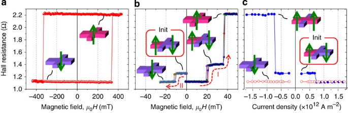
(A) main R–H curve. (for) small R–H Curves obtained after DW injection. Impedance curves with positive field sweep labeled I and negative field sweep labeled II were obtained after applying a DW injection pulse in the auxiliary field. HA of 0 and +27 metric tons, respectively. Each measurement was repeated five times. (C) Variation of Hall resistance with applied pulse current. Pulse current was applied with (closed blue symbols) and without (open red symbols) the DW preparation procedure. Schematic illustrations in A, for and C Visualize the magnetic configuration for each resistive state.
Current-induced DW characteristics
To examine current-induced DW motion, resistance versus current density (R–Y) The curve shown in Figure 2c It was measured by cycling through the following sequence: first, the DW was set at the initial location; Second, a current pulse of 10 ns length with variable amplitude and polarity was applied; Third, the Hall resistance was measured. Positive (negative) current is defined as a current that flows from left (right) to right (left). The change in resistance was also measured without the DW preparation process as a reference (open symbols). In DW configuration, the positive (negative) current reduces (increases) the Hall resistance with an amplitude greater than ±7 x 10¹¹ I am-2 while the resistance remains at the lowest state if no DW setting is performed. This indicates that the DW trapped at the Hall junction is displaced by the current pulse applied in the direction of electron flow, which is consistent with the DW motion induced by STT. We evaluated the temperature increase due to Joule heating and found that it was as low as 20 °C at a current density of 1 × 10¹² I am-2Even at DC, which indicates that it is negligible in the present experiment using nanosecond pulses (see Supplementary Figure S2 and Supplementary Note 2). Note also that the critical current density to move the DW to the right side becomes larger than that needed to move it to the left side as the pulse duration decreases to a few nanoseconds. This is due to the difference in the stabilization capability of the two DW movements, which will be discussed later. In what follows, we will focus on the dip of the DW caused by positive current injection, i.e. the dip to the left of the Hall junction.
Experiment on the probability of determining DW
Figure 3 The probability of selecting DW appears pTake off For different current densities and pulse durations, the pulse rise and fall time was less than 0.1 ns. To get pTake offThe measurement was repeated 100 times for each case. When the applied current density exceeds a certain threshold by about 10%, depth current removal becomes highly deterministic, i.e. 100 successes for 100 trials, for pulse durations longer than about 2 ns, whereas no removal is observed when the current density is below the threshold by about 10% (Figure 3a). Also the transmission pTake off From 0 to 1 with increasing current it becomes sharp when the pulse duration is longer than 2 ns (Figure 3b). Interestingly, the critical current density with respect to pulse duration is almost constant at durations longer than about 2 ns, while it increases significantly for periods less than 2 ns (Figure 3c). We will discuss the relationship between critical current density and pulse duration later. Figure 3D Shows 1-pTake offThat is, the specified error rate is 104 Repeat the same measurement sequence for 2 ns-long current pulses with different amplitudes. A small increase in current density above a certain threshold results in a sharp decrease in the error rate. It is also worth noting that no error was observed in No. 104 Experiments when the current density exceeds 8.5 x 10¹¹I am-2.
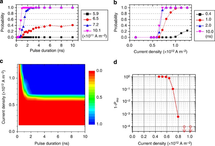
(A) pTake off As a function of pulse duration for four current densities. (for) pTake off As a function of current density for four pulse periods. (C) surroundings pTake off With current intensity and duration. (D) 1-pTake offThat is, determining the error rate as a function of current density. The pulse duration was 2 ns.
Calculate the probability of identifying DW
Let us consider the model that describes the probability of identifying DW shown in Figure 3. In order to reproduce the stochastic nature of the DW rotation, we took into account thermal fluctuations, which were also taken into account to describe CIMS at finite temperature.11,12. We used the one-dimensional Landau-Lifshitz-Gilbert equation, where the DW state is expressed by two mass coordinates (S, ϕ) represents the position and phase of the DW, and calculated the DW dynamics based on the equivalent stabilization potential25,(Figure 4a), (see Supplementary Note 3). The effect of thermal fluctuations is included as an initial distribution (S, ϕ) values (see Supplementary Note 4) and a random magnetic field that satisfies the fluctuation dissipation theory28(See Supplementary Note 5). We set each parameter to correspond to the current Co/Ni system (see Methods for details).
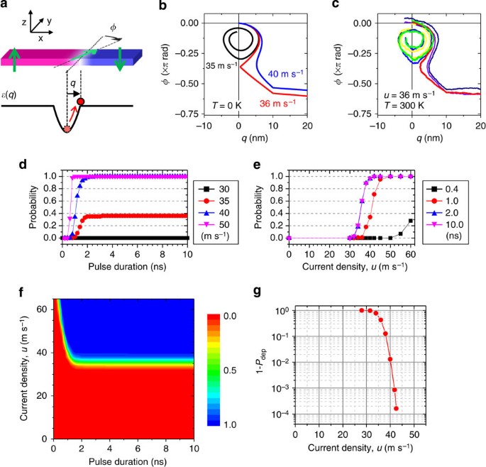
(A(parameter definition)S, ϕ) used in calculating the one-dimensional LLG. S is the position relative to the center of installation and ϕ is the magnetization angle DW, where the points of magnetization in the direction transverse to the wire, i.e. the Bloch wall case, are defined as ϕ=0. (for(path)S, ϕ) during current-induced DW removal without thermal fluctuations. Trajectories with three current density values are shown. (C(path)S, ϕ) with thermal fluctuations. Six paths with the same current density are shown. (D) pTake off As a function of pulse duration for four current densities. (e) pTake off As a function of current density for four pulse periods. (and) surroundings pTake off With current intensity and duration. (g) 1-pTake offThat is, determining the error rate as a function of current density. The pulse duration was 2 ns. To get pTake offthe calculation was repeated 100 times for (D–and) and 25,000 times for (g).
Figure 4b,c show paths (S, ϕ) after turning on the current without and with thermal fluctuations, respectively. With the current set of parameters, the critical current density ShC It is 36 m s-1at 0 K (Figure 4b). Figure 4c Shows six independent calculation results where current density and temperature are T It was 36 m s-1And 300 k. Three of them are proven and the others are not; This indicates the random nature of DW determination. Also, looking carefully at the paths, we can see that the initial distribution of (S, ϕ) and disturbances during the temporal development of (S, ϕ) affect whether a DW can be selected. For example, DWs start with a positive ϕ It generally tends to deviate, but the path shown by the green curve shows no deflection, although its initial state is similar to the red curve, which shows deflection. Figure 4d-g are the corresponding calculation results for Figure 3a–drespectively. Clearly, the calculation reproduces the trends observed in our experiment well; For example, the critical current density is almost constant when the pulse duration is higher than 2 ns, and the error rate drops sharply when the current density is slightly larger than a certain threshold value.